Excel COUNTIF function
The Excel COUNTIF function in the Excel table determines the number of items, based on the criterion we provide. The function can be used, as an example, for determining the quantity of supplies, stocktaking, etc. The manual assumes that we have basic knowledge of creating formulas in Excel.
Using the COUNTIF function in Excel
As already mentioned in the introduction, the Excel COUNTIF function does not provide the sum, but rather the number of cells based on the criteria that we selected. The Excel COUNTIF function syntax has the following arguments:
= COUNTIF (range of data compared , selection criteria)
The range of compared data may be defined using cell coordinates (e.g. A1:10) or using the name of the labelled field (labelled column, row, or dynamically labelled area). The criterion defines the cells that we wish to count. We can understand the Excel COUNTIF function better in the illustrated example:
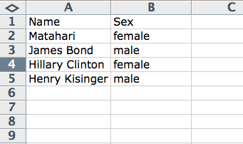
Our boss gave us the assignment of determining how many men (male) work in the firm from the employer roster, provided in the form of an excel table. Rewrite the following table into Excel:

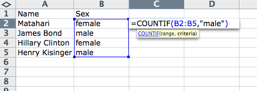
The solution is easy using the excel COUNTIF function. In C2, for example, we only need to enter the formula in the following form:
=COUNTIF(B2:B5,"male")
The formula works by passing through the range beginning with cell B2 and ending with cell B5. It counts the cells in this range that contain the word "man." The COUNTIF function thus calculates that two men work in the firm.

We do not use the parentheses if we are searching for a number. E.g., if we want to determine the number of cells that contain the number 1 in the range B2 to B5, then we write the formula in the syntax:
=COUNTIF(B2:B5,1)
Relational operators may be used in the COUNTIF function. For example, is equal to (=), is greater than (>), etc. The number of cells may also be determined based on two or more conditions. We might, perhaps, want to know the number of cells containing the number 1 and 2 in the range of B2 to B5. In that case, we write the formula in the following form:
=COUNTIF(B2:B5,1)+COUNTIF(B2:B5,2)
Excel COUNTIF functions - advanced processes
The Excel COUNTIF function is able to do far more than we have shown so far. In this chapter, we shall demonstrate advanced methods of using the Excel COUNTIF function. We shall learn how to calculate items based on the text string, which they contain. Everything is best understood on the illustrated example:
Our boss asks us to take an inventory of goods. Each good is labelled with a unique code. The code enables us to determine, e.g. what department the good belongs to, etc.
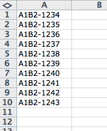
Before we begin solving the example, prepare the following table of inventory numbers in Excel:

The first letter of the inventory code indicates the department, to which the goods belong. Our first task is to determine how many items begin with the letter A. For this, we use the following formula:
=COUNTIF(A1:A10,"A*")
The asterisk (*) in the formula represents a text string. We have shown how to determine the first letter in the formula. Now we shall show how to determine the last letter of the inventory number. We may perhaps wish to determine, how many cells there are with 4 as the last number in the code:
=COUNTIF(A1:A10,"*4")
We only need to type an asterisk (*) before the character we are searching for. If we wish to know the number of cells that contain a B in any part of the text string, we need only to enter the formula in the following form:
=COUNTIF(A1:A10,"*B*")
We can also specify a search within text strings. Perhaps we may wish to count only the cells that have the letter B as the third-last character:
=COUNTIF(A1:A10,"**B*")
That was a small demonstration of how you can use the COUNTIF function in Excel to accomplish what at first glance seems impossible. If truth be told, the COUNTIF function in Excel is irreplaceable.
© Fotis Fotopulos, 2009
Pictures © Fotis Fotopulos, 2009