---

Labelling columns

Each table must be properly designed co that it serves us as much possible. We need to realize that new entries are constantly being added to the daily cash book. This means that the table is constantly expanding. We use column labelling to avoid having to constantly rewrite the formula into the newly added entries. The formula will thus automatically extend to the new entries entered into the table. The Excel SUMIF will save us a great deal of time when used in table designed in this manner. The instructions assume that you have basic knowledge of creating formulas in Excel.

Example:

The boss asks us to monitor entries and outgoing items - both separately. The accountant, however, insists that they must be together in a single table.

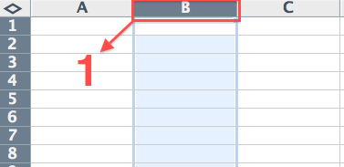
For viewing ease of this example, we shall only monitor entries and outgoing. We shall therefore label column B as "value":

1. Using the mouse, we click on column B, which selects the entire column (colours the column blue).
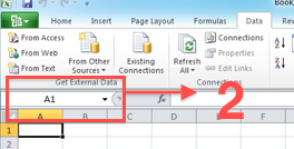
2. We type in the column label (left of the formula bar), in this case "value", and press the Enter key.

Using this simple procedure, we have labelled the first column into which we shall enter two values. Those values will be entries and outgoing. We then label as second, column C, as "cost." We shall enter the financial value of entries or outgoing into column C. After you have labelled the column, fill in the table using the data provided based on the example:

This is not the only method of labelling in Excel. In our case, we could have also used a dynamically labelled area, as also described in a different example on this webpage.

More informations about Excel

---

Excel SUMIF - example

The Excel SUMIF function literally invigorates a prepared table. This function enables the selection of only that data, which we need. Data selection, itself, is very simple. We only need to specify the condition in the SUMIF, according to which the data shall be selected.

The SUMIF function is recorded into the formula bar in the following manner:

=SUMIF(range,criteria,sum_range)

We use our example to demonstrate how to correctly enter the formula. We first add all of the entries from the table in the cash book. We display the sum of entries in cell E2.

1. The data range is column B2, which we labelled as "value."
2. The criteria is entry, which we write in the formula as ("entry") in parentheses. If the criteria is recorded in the cell, then we only need to write the cell designation, without parentheses.
3. Data shall be added from column C, which we labelled as "cost."

Insert the following formula into cell E2:

=SUMIF(value,"entry",cost)

If you entered the formula correctly, then the sum of all entries listed in cell E2 will be 800:

We shall now try to assign criteria in the formula as a cell reference. We shall calculate all outgoing:

1. Type "outgoing" into cell D4 - this will define criteria, which will be used to add outgoing from column B.
2. In cell E4, write the formula in the syntax =SUMIF(value,D4,cost).

If you entered the formula correctly, then the following table will appear:

Our overview of entries and outgoing items is finished. Our cash book now only needs a total balance. This can be calculated easily:

1. We can add cell E2 and cell E4.
2. We can alternatively use the SUM function, which we write in the form SUM(cost). We simply add the entire column, labelled as cost. Enter this formula into cell E6. Your table should then display as follows:

Our cash book now contains all necessary data. Now we only need to enter data into columns B and C (i.e. into the fields "value" and "cost"). These fields shall automatically expand themselves in the formula, and all three values shall automatically be calculated. This will provide constantly updated results without practically any work. On purpose, try and see how the Excel SUMIF function will save you time and streamline work.

We can achieve the same result using a PivotTable. Simply name the range and add it to the PivotTable.

More informations about Excel

© Fotis Fotopulos, 2009

Pictures © Fotis Fotopulos, 2009