Excel Formulas - free tutorial
Excel is a wonderful aid when calculating and analyzing data. In this chapter, we shall discuss procedures that order Excel to calculate numbers for us. This is done by writing a formula. For the formula to work, it must meet several rules. We therefore begin this chapter with the topic of Excel formula rules.
Excel formula and mathematics
Modifying a formula in Excel
Relationship between cells
Copying a formula within the table
Changing the result of the formula
Excel formula with function
Labelling a cell
Destination range in a formula
Excel formula rules
- Formulas are entered into cells in the same way as numbers or text.
- The formula is displayed in the Formula bar, where it may also be easily modified (it is labelled with the fx symbol).
- A formula must always begin with an equal (=) sign.
- A formula is created on the basis of mathematical rules.
- After pressing the Enter key, Excel only displays the result in the cell and the formula in the formula bar.

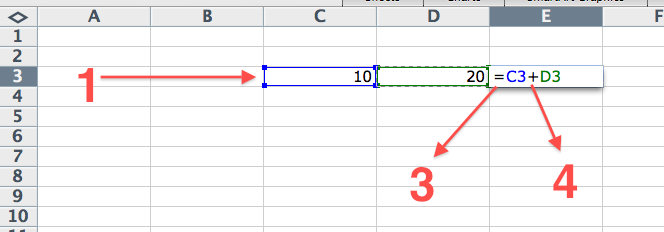

Excel formula and mathematics
We showed how to add two values in the example. We used the + sign, which is well known in mathematics. Remaining mathematical operations use the following signs in formulas:
+......................adding-..............subtraction
*..........multiplication
/......................divide
%.................percents
^.....................power
Modifying a formula in Excel
Demands change over time in every occupation, and we must similarly adapt Excel formulas to meet these demands (calculating expenses, monitoring revenues, tax calculations, etc.).
Example:
Revising a formula directly in the formula bar is the easiest. For example, we would like to add the number 10 to the formula.
Modifynig a formula in Excel step-by-step:
- We first click on the cell, to which the formula applies, using the mouse – i.e. cell D3. This displays the formula in the formula field.
- We click on the field and we can modify it using the familiar text cursor that appears. We simply add + 10 to the end of the formula.
- After revising the formula, we press the Enter key and the revised formula is saved, and the formula in cell D3 is immediately calculated.


Relationship between cells
In this chapter, we will show how Excel can be used to make work easier. It makes our work easier by calculating large quantities of numbers for us, without the need of entering them manually into a calculator. If we place the calculator aside and calculate everything using the formulas in the spreadsheet, we have significantly reduced our efforts in the future. If any situation changes, we need only to change the data and Excel calculates everything automatically. If we rely on a calculator, we would have to calculate everything from the beginning.
Assume that we are a car salesman and we create the following table, which we will also apply in the following examples (therefore, save it):

Example:
The end of the quarter is approaching and our boss asks us for the sales results of individual car models. Specifically then, how much cars of each model were sold over the last quarter.
First, we calculate the sales of Ford vehicles for the months of January + February + March, and we enter the result in cell E2:
- We click on cell E2 (selection indicated by bold frame).
- We write the formula =B2+C2+D2.
- After pressing the Enter key, the formula is calculated and the value 160 appears in cell E2.

Copying a formula within the table
Our table is finished. The first formula for calculating the sales of Ford vehicles is also finished. Now we only need to finish the sales for the remaining vehicles. Here is where Excel makes the work easier. We do not need to enter the formula for each vehicle separately; instead, we only copy the formula for Ford vehicles into the fields of remaining vehicles:
- Click on the cell E2.
- The cell border is displayed in bold, and a small box appears in its bottom right corner. We click on the box twice, and the formula calculates the result also for the other rows.

If we only wish to calculate certain rows, then we only click once on the box while holding the button and dragging the mouse into the row we select. We then release the button, and the formula is calculated.

Changing the contents of the cell will also change the result of the formula
Our sales results are finished and we wish to send them to our boss. A sales representative, however, informs us that he sold one extra Ford. The solution is easy. We do not need to recalculate anything, but only revise the number in the appropriate cell. We only need to revise the input data and the formula automatically recalculates the result.
Table prior to revision:

Revised table:

Excel formula with function
Excel formulas often use functions. We will thus demonstrate how to insert them into formulas.
Example:
Our boss would like us to calculate how many cars were sold in total.
The easiest way of accomplishing this is by using the SUM function:
- We select cell G2.
- We type in it the formula =SUM(E2:E6).

The SUM function has its own tutorial. The explanation of the formula will thus be brief. SUM adds together the selected cells. In our case, it adds the column that begins with cell E2 and ends with cell E6 (outlined in blue on the picture).
Labelling a cell
Tables and calculations are easier to view when we label the cells ourselves. With Excel, we can name a cell as we wish and use this name when calculating formulas.
Let us label the cell G2 as sum:
- We select the cell G2 by clicking on it (boldly outlined).
- Overwrite G2 to sum in the name box and press Enter. The name box is located left of the formula bar.
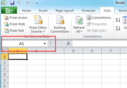
We can use the labelled cell in formulas for calculations just as any other. Instead of G2, we write sum in the formula. We demonstrate in a simple formula. We wish to multiply the total number of sold cars (given in the cell, labelled sum) twice, e.g. by the number in cell H2:
=2*(sum)
In Excel, we can label not only a cell, but even an entire row, if desired. We can also label an entire column, or a series of cell that we select directly. A superior feature is dynamic labelling, which automatically expands the area by new entries in the table.
An additional note in conclusion: Destination range is used in cell labelling of formulas. This means that the referenced cell remains unmodified when copying a formula.
Destination range in a Excel formula
Destination range means that a cell never changes when copying a formula. We demonstrate the principle on the following example:
Your boss asked you to prepare a daily current price list of vehicles in several currencies (for example, in dollars, Swiss francs, and rubbles).
We are using Excel, so we are not going to slave every day over a calculator. It suffices that we know how to work with a table and how to create formulas, so we may begin our task without fear.
Prepare and save the following table:
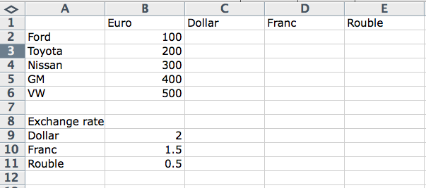
We shall label cells A9 to A11 according to the names of currencies, and we shall fill in the current values of these currencies into these cells.
We have prepared our table of currencies, and we can therefore begin writing formulas:
- Formula for converting to the dollar amount is written =B2/dollar.
- We place the formula into cell C2.
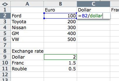
We apply the formula in cell C2 (cost calculation of Fords in dollars) to all vehicles. We notice that the cell labelled dollar does not change in the formulas of remaining cars. That is the advantage of the destination range. If instead we use the source range, then the cost of the Toyota in the third line will be calculated in francs instead of dollars.
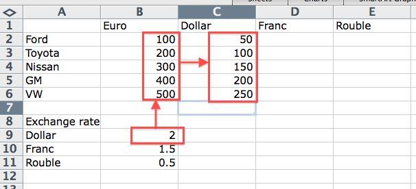
We calculate the prices for other currencies in the same manner:
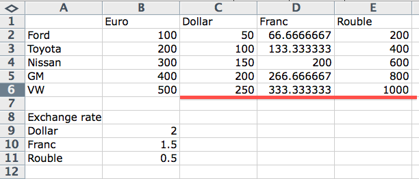
The spreadsheet is now ready. We only need to come to work every morning and find out the current exchange rate. We insert the current exchange rate into the correct cell, and Excel calculates everything by itself. We can use the time we saved to make some coffee or to learn a second method of assigning destination ranges using the $ (dollar) sign. We will demonstrate this in the next example:
While our boss is satisfied that he has a current price list of vehicles every day in several currencies, he just remember that he wants a list of quarterly revenues. In fact, he needs the revenues of individual vehicle models for every month separately.
We copy our original table into our spreadsheet and create the following table below it:
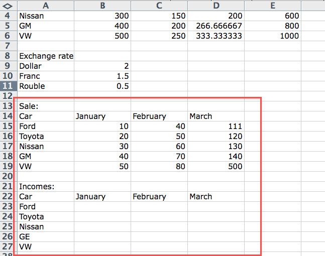
In cell B23 we write the formula =B2*B15, which we apply to the remaining cells:
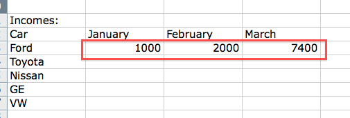
The result in cell B23 is correct, but the other cells display outright nonsense. This happened because we did not use the dollar $ to fix column B, which lists the costs of vehicles. We therefore revise the formula into the correct form and again copy it across all months:
=$B2*B15
All sales revenue values in the table are now correct and we finish calculating the entire table:

This picture shows how to select a column. We accomplished this by using the symbol $B2; however, it occasionally happens that we need to set a row instead of a column when performing the calculation. This can be done very easily. We move the dollar sign between the dollar and number so it reads B$2. In this manner, we effectively set the row.
We did not select this final example by chance. The calculated results show us how much work Excel can save us. We can now easily create price lists in individual currencies. We already know how to do this -- we only need to overwrite the exchange rate of each currency in the cells, which are labelled according to their names of currencies. We have prepared a table for calculating revenues, which saves us further work. Here comes the best part. The calculations in the tables are interconnected, and this will save us a great deal of additional work. Imagine that the cost of cars changes every day. A manual calculation would take up an unbelievable amount of time, but since the calculations in the table are only related within individual cells, we revise the current costs of vehicles and Excel calculates everything for us. It calculates for us not only the foreign currency conversion, but it also calculates the revenues.
© Fotis Fotopulos, 2009
Pictures © Fotis Fotopulos, 2009